Why grow a plant you can't eat
Measuring a plant is harder than it sounds. Height is easy enough with a ruler. Leaf area is not: the honest way to get it is to cut the plant down, pull off every leaf, and run them through a scanner. You get one number, and you no longer have a plant. Count the leaves on a mature cowpea and you will undercount, because the lower canopy is hidden underneath the upper one.
A simulated plant has none of those problems. Every leaf is a known object at a known position with a known area. Nothing is hidden, nothing is destroyed, and measuring it costs nothing.
That gap is the whole point. Simulation isn't here to replace the field — it's here to give you a world where the answer is already known, so you can check whether your field methods would have found it.
The one idea to take away: these quantities are free and exact in simulation, expensive and noisy in the field. Simulation-driven phenotyping exists to trade on that asymmetry — use the free-and-exact world to build and test the tools that have to survive the expensive-and-noisy one.
A stage and its departments
Before any code, one mental model. Helios is organised like a theatre production.
At the centre is the Context — the stage. It holds every piece of geometry in the scene as primitives: small triangles and patches. Each primitive can carry named data of its own — how much light it absorbed, its temperature, which organ of which plant it belongs to.
Around the stage sit the plug-ins — the departments. The plant-architecture plug-in writes geometry onto the stage: it grows plants. A radiation plug-in reads that geometry and writes back absorbed-light values. An energy-balance plug-in reads those and writes temperatures.
The rule that makes this work: no plug-in talks to another plug-in. They only read and write data on the primitives. That indirection is what lets you bolt on physics later without rewriting anything.
Why this matters now rather than later: because everything communicates through primitive data, any model you add afterwards works on the plant you build today. The cowpea is the reusable asset, not the throwaway.
Setup
pip install pyhelios3d
That's the whole installation. The wheels ship with prebuilt native binaries — underneath the Python API sits the actual Helios C++ core, so nothing needs compiling.
You do not need a GPU for any of this. Ray-traced radiation is where CUDA eventually earns its keep, and that comes later in the series. Growing geometry and measuring it is all CPU work.
Growing the plant
Here is the entire thing. Six meaningful lines.
from pyhelios import Context, PlantArchitecture
from pyhelios.types import vec3

with Context() as ctx:                          # ①
    with PlantArchitecture(ctx) as pa:          # ②
        pa.disableMessages()                     # ③
        pa.loadPlantModelFromLibrary("cowpea")   # ④
        pid = pa.buildPlantInstanceFromLibrary(  # ⑤
                  vec3(0, 0, 0), 0)
        pa.advanceTime(35)                       # ⑥ days
- ① Context() as ctx
- Creates the stage. It's a context manager because the geometry lives in native C++ memory rather than Python's, and the
withblock guarantees that memory gets released. This is also why every query has to happen inside the block — once it exits, your handles point at freed memory. - ② PlantArchitecture(ctx)
- Attaches the growth department to this particular stage. Passing
ctxis the wiring: everything the plug-in builds lands in that Context's primitive store. - ③ disableMessages()
- Silences the plug-in's progress chatter. Purely cosmetic, but in a notebook it's the difference between readable output and a wall of log lines.
- ④ loadPlantModelFromLibrary("cowpea")
- Loads a parameterised species description — and this is the part worth slowing down on. It is not a mesh. It's a bundle of rules: internode lengths, leaf-angle distributions, branching probabilities, the thresholds at which the plant changes developmental stage. Call
pa.getAvailablePlantModels()to see the rest of the library — bean, sorghum, maize, tomato and others. - ⑤ buildPlantInstanceFromLibrary(vec3(0,0,0), 0)
- Instantiates one plant from those rules, at the origin. The second argument catches people out: it's the plant's starting age in days, not a random seed. You get back
pid, the handle every later query needs. - ⑥ advanceTime(35)
- The line doing all the work. Thirty-five simulated days pass.
Growth is procedural, not a mesh being scaled. Over those 35 days the model initiates nodes at a development-driven rate, elongates internodes, unfolds leaves along the species' angle distributions, and branches into new shoots. Stop at day 20 and you get a genuinely younger plant — fewer organs, different architecture — not a shrunken copy of the day-35 one.
Measuring it like a phenotyping rig
The plant exists. Now interrogate it — still inside both with blocks.
        print("primitives :", ctx.getPrimitiveCount())
        print("leaves     :", len(pa.getPlantLeafObjectIDs(pid)))
        print("shoots     :", len(pa.getAllShootIDs(pid)))
        print("age        :", pa.getPlantAge(pid))
        print("height     : %.2f m" % pa.getPlantHeight(pid))
        print("leaf area  : %.3f m2" % pa.getPlantLeafArea(pid))
primitives : 53634
leaves     : 272
shoots     : 11
age        : 35.0
height     : 0.46 m
leaf area  : 0.606 m2
Read those the way a breeder would. Every one is a trait — and every one has a price tag in the real world.
| value | reads as | what it costs in the field |
|---|---|---|
| height 0.46 m | plausible day-35 cowpea stature | drone surface model minus ground model — needs photogrammetry and centimetre-accurate georeferencing |
| leaves 272 | organ count across the whole plant | essentially unmeasurable at scale — occlusion hides the lower canopy |
| leaf area 0.606 m² | the light-capture engine; the per-plant cousin of LAI | destructive harvest and a leaf scanner, or a model-based estimate carrying real uncertainty |
| shoots 11 | branching architecture | hand-counting, plant by plant |
| primitives 53,634 | the triangles the plant is built from | no field equivalent at all |
Those 53,634 primitives aren't trivia. Each one can carry data — absorbed radiation, temperature, water status — which is what makes this same plant the substrate for every physics post later in the series.
Looking at it
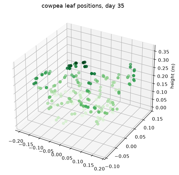
Numbers are the point, but it helps to see the thing you grew.
        bases = pa.getPlantLeafBases(pid)        # still inside the with-blocks!
        xs, ys, zs = zip(*[(b.x, b.y, b.z) for b in bases])

import matplotlib.pyplot as plt                  # plotting can happen outside
fig = plt.figure(figsize=(6, 7))
ax = fig.add_subplot(projection="3d")
ax.scatter(xs, ys, zs, c=zs, cmap="Greens", s=30)
ax.set_zlabel("height (m)")
ax.set_title("cowpea leaf positions, day 35")
plt.show()
What the dots are — and aren't
getPlantLeafBases returns the coordinate where each leaf's petiole meets its stem. One dot per leaf, 272 in all. So the dots are attachment points, not leaves — the actual leaf surfaces live in the primitives, angled and overlapping one another.
Which makes this modest figure quietly interesting. It is a small, perfectly labelled point cloud — the same data structure a LiDAR scanner produces — except here every point is known and nothing is occluded. That is exactly the setup you need to ask what a real scanner would have missed.
Where this goes
You now have a plant that is fully known: every organ, every position, every area. The next step is to stop trusting that knowledge and start testing instruments against it — scanning this same cowpea with a simulated laser, and measuring precisely what the scan fails to see.
That is the loop the whole section runs on. Build a world where the answer is known, then find out which of your methods can recover it.